A Lean Six Sigma Master Black Belt was perplexed by the software’s correlation and regression analysis output. The results were pure nonsense. In addition to regression coefficients that were negative when common sense told him they should be positive (and vice versa), some of the correlation coefficients were large, while the corresponding regression coefficient p-values were insignificant. What the heck was going on?
The problem with the Master Black Belt’s data was multicollinearity, a condition that’s encountered more often as Six Sigma practitioners move from engineering and manufacturing data to customer survey data.
Multicollinearity refers to linear intercorrelation among variables. Simply put, if nominally “different” measures actually quantify the same phenomenon to a significant degree–i.e., the variables are accorded different names and perhaps employ different numeric measurement scales but correlate highly with each other—they’re redundant.
Multicollinearity isn’t well understood by the applied statistics community. Researchers at Arizona State University found widespread misunderstanding of multicollinearity and other regression analysis concepts among graduate students who had taken, on average, five graduate and undergraduate statistics courses. I’ll try to explain multicollinearity by using a simple, everyday metaphor: a table.
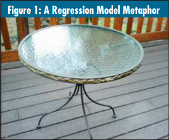
Consider the photograph of a table shown in figure 1. This is a finely built table I purchased at Wal-Mart for only $99 (chairs were included). In my metaphor, the table is a model. The legs of the table represent x variables, or predictors. The top represents the y variable, the predicted variable. My intent is to build a table where the top is well supported by the legs, i.e., the predictions are well explained by the predictors.

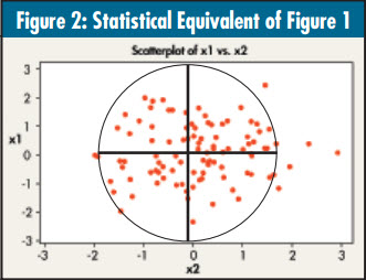
The table legs are placed at 90° to each other. This angle provides maximum support for the top. In statistics, when two variables are uncorrelated with each other, they’re said to be orthogonal, or at 90° to one another. If you create a scatter diagram of two uncorrelated variables and draw best-fit lines, you get something that looks like figure 2: The lines are at 90° to one another.

Consider the two x variables to be the legs of the table, the circle to be the table top and the dots to be objects on the table’s surface. You can see that the x variables do a good job of “supporting” the y variable. If you add a few dots anywhere within the circle they’re unlikely to make the table tip over. In other words, the model is stable.
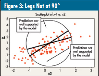
What if the table wasn’t built with the legs at 90°? Clearly, it wouldn’t be as stable. The statistical equivalent to this poorly designed table is shown in figure 3. The lines no longer cross each other at 90° because the two x’s are correlated with one another. There are areas within the circle (i.e., our y model and the equivalent of the table top) that aren’t well explained by the model. If we take additional samples and get y’s in either of these regions, the coefficients of the model will change drastically, i.e., the model, like the table, will be unstable. This is the multicollinearity problem in a nutshell.

Using our table metaphor, we can see that regression models are more stable when the x’s used to predict the y are uncorrelated with one another. If the x’s are correlated, there are a number of statistical techniques that can be used to address the problem. When many x’s are involved, I like to use principal components analysis, which replaces many correlated variables with a smaller number of uncorrelated factors. This not only overcomes the problem of multicollinearity, it usually also makes the model easier to understand and use.

Leave a Reply